Microbial association network construction tutorial

Disclaimer: Note that results may look a bit different for the 2017 version of the arctic soil data.

So far, we have presented 4 different ways to infer a microbial association network. Here, we will demonstrate how the network can be analysed. For convenience, we will describe network analysis steps in Cytoscape on the network generated with CoNet, but there are many other options for network analysis, such as the tools offered by MENA, igraph in R or NeAT (in NeAT's link section, you can find many more network analysis platforms).

Step 0 - Compare results between MENA and CoNet
Before analyzing the CoNet network, we will compute the extent of agreement with the MENA network. Since this requires some data parsing with a text editor capable of advanced string replacement, you may skip this step.
First, save the CoNet network as sif file (here named conetNetwork.sif). Open conetNetwork.sif and replace the tab-dash-tab separator between its two columns by the separator between the two columns of the MENA sif file, such that a line in the conetNetwork.sif file looks like this:

OTU-531025	pp	OTU-364090
 

Then load the sif file again into Cytoscape. This parsing step makes edge names between the MENA and CoNet networks comparable.
We can now proceed to the computation of the network intersection. For this, open Tools->Merge Networks and select "Intersection", then select the parsed CoNet and the MENA network and finally click "Merge". The intersection between the two networks is quite small (only a few edges appear in both networks).

Step 1 - Global network analysis
To compute global network properties in Cytoscape 3.X, click on Tools->Network Analyzer->Network Analysis->Analyze network. A panel asks you whether or not the network is undirected. With the selected configuration, CoNet outputs an undirected network. Do you know why? (You can find an explanation here). Once you click OK, you will be given an overview panel with network parameters such as network diameter, density, characteristic path length and clustering coefficient. The plot below shows the node degree distribution. The goodness of fit of a power law to this distribution is a measure of the scale-freeness of the network. Node-specific properties (such as eccentricity and betweenness centrality) are also computed, which are added as additional columns to the node property table.

Step 2 - Hub nodes
A popular analysis type is to look at the nodes with the largest number of connections. CoNet assigns the degree (number of edges connected to a node) as well as the positive degree (number of positive edges connected to a node) and the negative degree (number of negative edges connected to a node) to each node. As an exercise, you can find out which node is connected to the largest number of positive or negative edges by playing around with the node property table. Please click here for a solution. In the arctic soil network inferred with CoNet, the top connected node belongs to the Acidobacteria and is also the top negative hub. The top positive hub also belongs to the Acidobacteria. However, even the positive hub has several negative edges.
Please note that when several networks with the same node names are open, Cytoscape displays the properties of a node in one network, but does not update it when another network containing the same node is selected. To make sure the right node properties are displayed, restore the CoNet network in a fresh instance of Cytoscape. Here is an explanation on how to restore an already computed network with CoNet.

Step 3 - Network clustering
In gene expression networks, clusters are detected in order to suggest a function for genes with unknown functions relying on the "guilt by association" principle: if the gene clusters together with other genes of known function, its function is predicted to be similar to that of its neighbors. In the context of microbial association networks, clustering can help uncover similarities in life style, as done by Chaffron et al. in Genome Research 20, 947-959 (2010), where the network was clustered with MCL. We will use the OH-PIN algorithm instead.

Before clustering the network, we will select positive edges. You can think about the reason for this (an answer is provided here).
There are two ways to select positive edges; one involves Cytoscape's functionality and the other CoNet's restore capabilities. As an exercise, you can try to find the Cytoscape (3.X) functions that carry out this task. Click here to see a solution. Alternatively, you can restore a positive-edge-only network from the random score files. For this, you can follow the restoration procedure explained here. Before you launch the re-computation with "GO", enable "copresences only" in the Preprocessing and filtering menu.
The resulting network consisting only of the positive edges forms several connected components. You can also deduce from the edge numbers of the original network and the positive-edge-only network that the arctic soil network inferred with CoNet has more negative than positive edges.

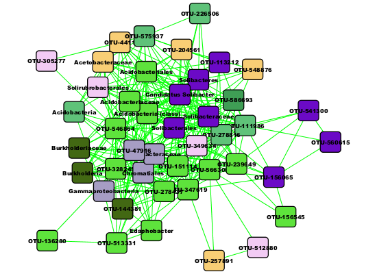
We will now cluster the positive-edges-only network using the Cytoscape plugin CytoCluster. You can open CytoCluster via the App menu. Select the OH-PIN algorithm with default values and run it by clicking on "Analyze current network" in the CytoCluster panel. CytoCluster displays the resulting clusters in an extra panel. With the selected settings, CytoCluster detects several clusters, 2 big ones and a few smaller ones. We can now click at the first cluster in the CytoCluster result panel and analyse it phylogenetic composition on the class level by selecting "class" as "Node Attribute Enumerator". The first cluster is composed mainly of Acidobacteria and Solibacteres. We can instantiate it as a separate network by clicking "Create Sub-network". 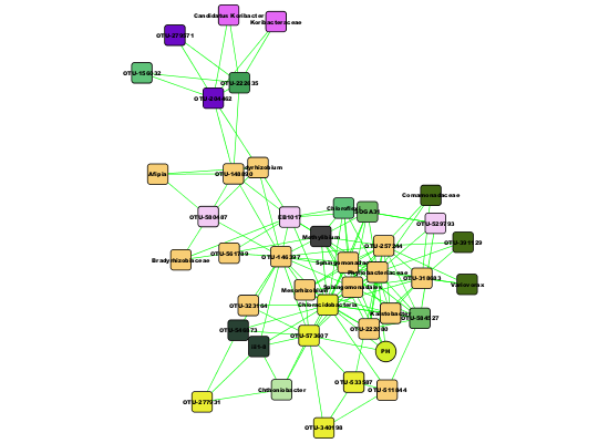The second cluster mainly consists of Alphaproteobacteria and Chloracidobacteria.





Step 4 - Neighbors of environmental parameter
We can now look at the neighbors of the pH node, which represents the only environmental property that we included in the network inference. Since it is an environmental property, CoNet assigned this node another shape than the taxon nodes. When we select the first neighbors of the pH node, we find a sub-network looking similar to the one below:


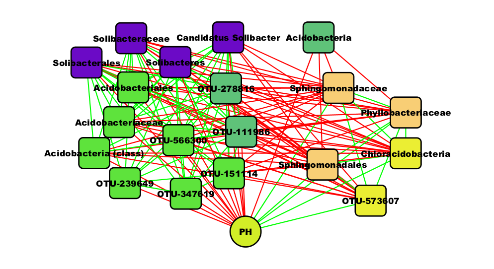
You can think about the biological interpretation of this sub-network. More details are given in the conclusions.