SPIEC-EASI
SPIEC-EASI (SParse InversE Covariance Estimation for Ecological Association Inference)
exploits the fact that under certain assumptions (that all relevant variables are being considered
and the data are multivariate normally distributed),
the inverse covariance matrix corresponds to a network without indirect edges. In a nutshell,
SPIEC-EASI estimates the inverse covariance matrix
from sequencing data. The inference of networks using the inverse covariance matrix is also
known in the literature as Graphical Gaussian model
and the inverse covariance matrix is also referred to as precision or partial correlation matrix.
SPIEC-EASI is implemented in R, thus
for this tutorial, we will work with R. By the way, the SPIEC-EASI package also provides an
alternative implementation for SparCC. For details of SPIEC-EASI, please check out
PLoS Computational Biology 11(5) e1004226.
Note: We will run SPIEC-EASI on the 2017 version of the arctic soil data set stored in Qiita (see CoNet 2017 tutorial).
Credit: This tutorial makes use of some commands suggested in this SPIEC-EASI tutorial.
Step 1 - Installation and biom format conversion
Please install the R package SpiecEasi by typing the commands below in R. If you do not have the devtools R package, please install it first using command: install.packages("devtools")
library(devtools)
install_github("zdk123/SpiecEasi")
library(SpiecEasi)
Next, install the R package phyloseq:
source('http://bioconductor.org/biocLite.R')
biocLite('phyloseq')
library(phyloseq)
And finally, the R package seqtime:
install_github("hallucigenia-sparsa/seqtime")
library(seqtime)
Next, we prepare our data for loading into R. The 232_otu_table.biom file that we obtained from Qiita is in HDF5 format. Phyloseq supports the JSON format of biom instead, therefore we have to convert the original biom file into json format using the biom converter. The command is:
biom convert -i 232_otu_table.biom -o arctic_soils_json.biom --to-json --table-type="OTU table"
You can also download the json-formatted biom file here.
Step 2 - Data import and preprocessingFirst, we tell R in which folder the arctic_soils_json.biom file is located. Below, an example path is given (please enter your real path). Note that in Windows, the path separator is a backslash instead of a slash.
input.path="/Users/SPIECEASI/Input/"
output.path="/Users/SPIECEASI/Output/"
biom.path=file.path(input.path,"arctic_soils_json.biom")
We can then load the biom file with phyloseq function import_biom. We extract the OTU table with OTU abundances and the taxonomy table from the resulting phyloseq object.
phyloseqobj=import_biom(biom.path)
otus=otu_table(phyloseqobj)
taxa=tax_table(phyloseqobj)
The OTU matrix contains many OTUs that are zero in almost all samples. As in CoNet, we filter these OTUs, but keep their sum so as not to change the overall sample counts. We will do this using seqtime's function filterTaxonMatrix. We keep the indices of filtered OTUs to remove their corresponding entries in the taxonomy table. In addition, we introduce dummy taxonomic information for the last row of the filtered OTU table, which contains the sum of the filtered OTUs. We also give this row a dummy OTU identifier.
filterobj=filterTaxonMatrix(otus,minocc=20,keepSum = TRUE, return.filtered.indices = TRUE)
otus.f=filterobj$mat
taxa.f=taxa[setdiff(1:nrow(taxa),filterobj$filtered.indices),]
dummyTaxonomy=c("k__dummy","p__","c__","o__","f__","g__","s__")
taxa.f=rbind(taxa.f,dummyTaxonomy)
rownames(taxa.f)[nrow(taxa.f)]="0"
rownames(otus.f)[nrow(otus.f)]="0"
Next, we assemble a new phyloseq object with the filtered OTU and taxonomy tables.
updatedotus=otu_table(otus.f, taxa_are_rows = TRUE)
updatedtaxa=tax_table(taxa.f)
phyloseqobj.f=phyloseq(updatedotus, updatedtaxa)
Step 3 - SPIEC-EASI Run
Now we are ready to run SPIEC-EASI. SPIEC-EASI will take care of normalization, thus we do not
preprocess the OTU table beyond the filter step.
SPIEC-EASI's method parameter specifies the method used to compute the
sparse inverse covariance matrix. The default is glasso, but we will use here the faster alternative mb,
which stands for meinshausen-buhlmann neighborhood selection.
Both inverse covariance matrix estimation techniques involve the estimation of a penalty parameter, which
counteracts overfitting (thus enforcing sparsity, i.e. networks with few edges). SPIEC-EASI estimates this penalty
parameter using a form of bootstrap called Stability Approach to Regularization Selection (StARS).
StARS consists in repeating the inference on random sub-sets of the data and selecting the penalty parameter such
that the resulting network is least variable across repetitions. The number of these repetitions is given by rep.num.
Note that in this example case, even after the filtering step, we have less samples (52) than OTUs (188). Thus,
the famous n << p situation applies: our sample number n is smaller than our dimensionality p. SPIEC-EASI can solve
the network inference problem regardless, by relying on the sparsity assumption, i.e. on the assumption that only
few interactions exist. Ideally, SPIEC-EASI should be applied to data sets with many more samples than OTUs.
spiec.out=spiec.easi(phyloseqobj.f, method="mb",icov.select.params=list(rep.num=20))
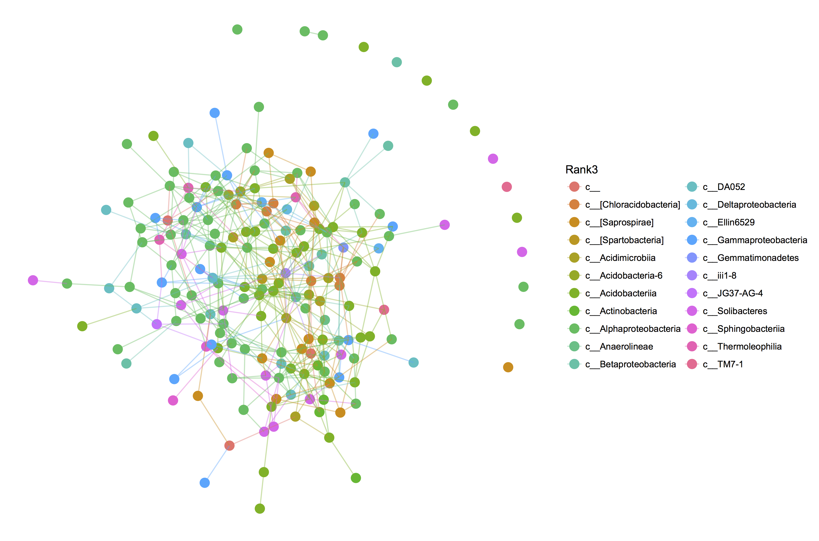
Next, we convert the output of SPIEC-EASI into a network and plot it with colors on class level (which is the 3rd level in the default seven-level taxonomic hierarchy). If assumptions are met (all relevant variables taken into account, data multivariate normally distributed), an absence of an edge (a zero) means that two species do not interact directly.
spiec.graph=adj2igraph(spiec.out$refit, vertex.attr=list(name=taxa_names(phyloseqobj.f)))
plot_network(spiec.graph, phyloseqobj.f, type='taxa', color="Rank3", label=NULL)
For more recent versions of SPIEC-EASI, please try the following command to obtain the network:
spiec.graph=adj2igraph(getRefit(spiec.out), vertex.attr=list(name=taxa_names(phyloseqobj.f)))
Please see here for more help on the recent SPIEC-EASI version.
The resulting network plot is shown below.
Step 4 - SPIEC-EASI Analysis
First, we would like to know how many positive and negative edges SPIEC-EASI inferred. The inverse covariance matrix is obtained via a form of regression. The first step to count positive and negative edges is thus to extract the regression coefficients from the SPIEC-EASI output, which for method mb is achieved with command getOptBeta. The regression coefficient matrix is not symmetric and can be symmetrised with command symBeta.
betaMat=as.matrix(symBeta(getOptBeta(spiec.out)))
We can then obtain the number of edges in the network from the matrix of regression coefficients. Please try to do it yourself. A solution is provided here. As an advanced exercise, you can also try to visualize the SPIEC-EASI network with positive and negative edges colored differently using igraph. A rough solution to this problem is available here.
Next, we will cluster the SPIEC-EASI network and list the taxa present in each cluster. The R package igraph (installed as a dependency of seqtime) offers a number of graph clustering approaches. Here, we run a quick, greedy clustering algorithm and then extract the cluster memberships from the output object.
clusters=cluster_fast_greedy(spiec.graph)
clusterOneIndices=which(clusters$membership==1)
clusterOneOtus=clusters$names[clusterOneIndices]
clusterTwoIndices=which(clusters$membership==2)
clusterTwoOtus=clusters$names[clusterTwoIndices]
When summarizing and sorting the representatives of the different classes, we see that the first cluster is dominated by Saprospirae and Acidobacteriia and the second by Alphaproteobacteria.
sort(table(getTaxonomy(clusterOneOtus,taxa.f,useRownames = TRUE)),decreasing = TRUE)
sort(table(getTaxonomy(clusterTwoOtus,taxa.f,useRownames = TRUE)),decreasing = TRUE)
As an advanced exercise, you can try to repeat clustering without negative edges.
A solution is provided here.
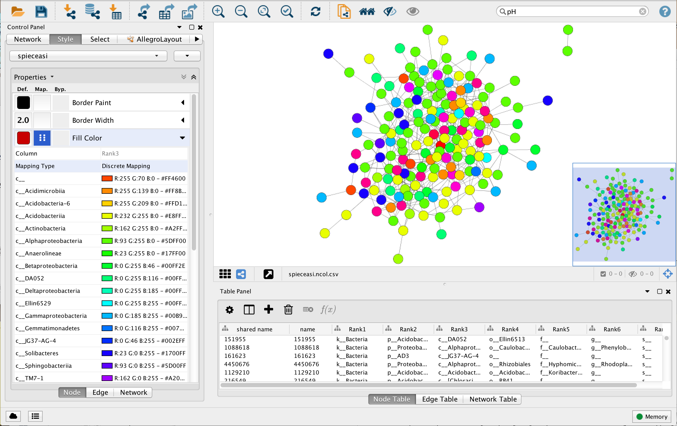
Step 5 - Importing into Cytoscape
The igraph R package allows exporting graphs as edge lists, which can be imported into Cytoscape.
As an exercise, you can try to import the SPIEC-EASI graph into Cytoscape using igraph's
write.graph function. Please use an export function that preserves the OTU identifiers.
You can find the solution to this task here.
Next, we will export the taxonomic information, so we can load them onto the nodes in Cytoscape.
write.table(taxa.f,file=file.path(output.path,"arctic_soil_lineages.txt"),sep="\t", quote=FALSE)
You need to manually edit the resulting file to add a header to the first column with the
OTU identifiers. This can be done by writing OTU followed by a tab in the beginning of the
first row.
In Cytoscape, open File -> Import -> Table to select the file and click OK. This should automatically
load the taxonomic information onto the nodes.
You can now create a new style by going to Style -> Create New Style. You can for instance
name the new style spieceasi. Try to color the nodes according to their class.
Once the network is imported into Cytoscape, you can run the NetworkAnalyzer (described
in the Network Analysis section) to compare
its properties with the properties of the CoNet network.