CoNet (2017)
This is an updated version of the CoNet tutorial presented in 2014.
CoNet offers ensemble-based network construction, i.e. several similarity
measures can be combined. The basic ensemble approach and the ReBoot technique used to
alleviate compositional bias is explained in
PLoS Computational Biology 8 (7), e1002606. The CoNet app has also been published in
the F1000 Cytoscape app channel here.
Since this tutorial is presented by CoNet's developer, CoNet is explained more intensively
than the other tools.
Step 1 - Data
You can skip this step and download required data files directly from here.
The QIIME database has now become the Qiita database. We will download the arctic soil data
from the Qiita database. Please log into the Qiita database and enter the query "arctic soil".
Select the study with identifier 104. This should open a screen like this one:
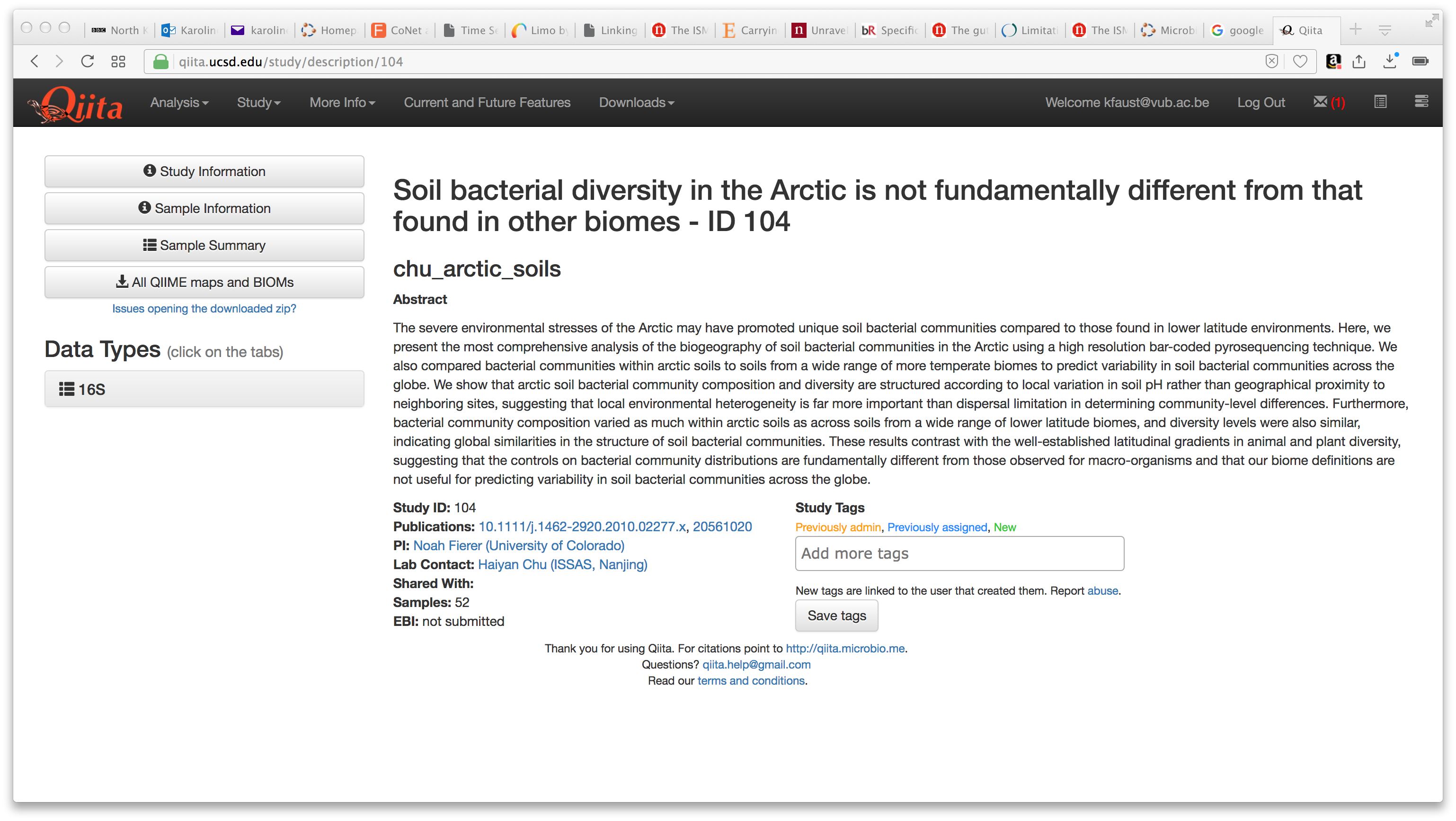
Please click "All QIIME maps and BIOMs" to download the tutorial files.
This will download a folder with sub-folders BIOM, mapping_files and processed_data. We will
work with files 232_otu_table.biom in processed_data and 2607_mapping_file.txt in mapping_files.
CoNet can work with the biom file directly. However, we have to extract features of interest
from the mapping file. For this, you can open this mapping file in Excel and copy the "#SampleID" column and
the "PH" column into a new sheet, with the "#SampleID" column as first and the "PH" column as second column.
Then remove the # from the "#SampleID", since # is interpreted as starting character of a comment line.
You can then save the two columns into a tab-delimited file. We will refer to this file as "arctic_soils_features.txt".
Step 2 - Basic configuration
All the following steps assume that you are working with Cytoscape 3.X. If you use Cytoscape
2.X, you can convert the biom file into an OTU table using the
biom converter
or download the OTU table here.
In the CoNet configuration, you have then to enable "Table obtained from biom file" instead
of "Biom file in HDF5 format" in the Data menu.
You can skip this step and proceed to the next, if you use
the conet-permut-settings.txt file
instead of configuring CoNet manually.
Data
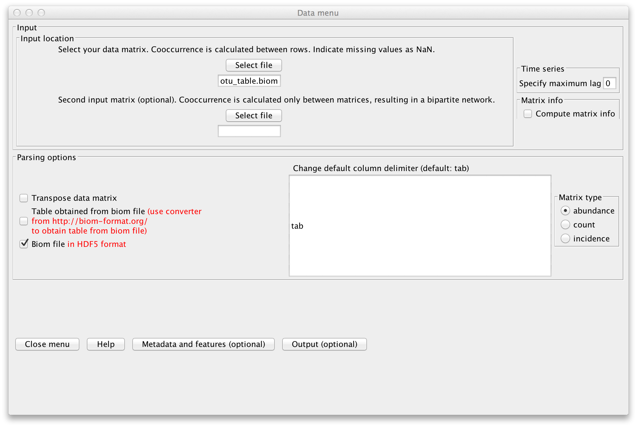
Open the CoNet app in Cytoscape. Open the "Data" menu and load the "232_otu_table.biom" file
that contains the lineages. Enable "Biom file in HDF5 format".
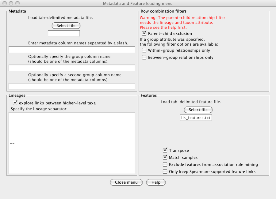
Open the "Metadata and Features" sub-menu and enable
"explore links between higher-level taxa". This will cause CoNet to assign higher-level taxa
from the lineages, e.g. "Solibacterales". Also enable "Parent-child exclusion" to prevent
links between higher- and lower-level taxa of the same lineage, e.g. between Acidobacterales
and Acidobacteriaceae.
Finally, load the "arctic_soils_features.txt" file via the "Select file" button in
the Features part of the "Metadata and Features" sub-menu and enable "Transpose"
and "Match samples". CoNet will transpose the environmental parameter file such
that rows become columns and vice versa and will in addition match the sample names
(discarding samples that are not present in both files), such that samples in the
OTU file and in the environmental parameter file have the same order.
Preprocessing
Rare taxa need to be discarded, since their presence and absence is depending more on the sequencing
depth than on biological reasons. In addition, sequencing depth differences can introduce
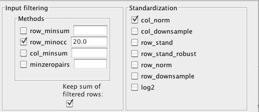
spurious correlations. We lump all taxa below a minimum occurrence of 20
across the samples into a garbage taxon and convert counts into relative abundances by opening the
"Preprocessing and filtering menu" from the main menu and enabling "row_minocc" with value 20,
"Keep sum of filtered rows" and "col_norm".
Methods and thresholds
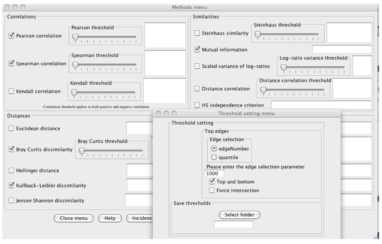
In the "Methods menu", we select 5 methods for the ensemble inference: Pearson,
Spearman, Mutual Information, Bray Curtis and Kullback-Leibler dissimilarity. Instead of specifying
their thresholds manually, we request the 1000 top edges for each method in the
"Threshold setting menu", where we also enable "Top and bottom" (to retrieve the 1000 top
negative correlations as well).
Run
If you now click "GO" in the main menu, a multigraph with at least 5*2*1000 edges will be constructed
(5 methods, top and bottom, 1000 top edges). There can be more edges in case of ties (scores of equal value).
This is the initial network, which will be refined by randomization. Positive edges are automatically colored in green,
whereas negative edges are colored in red. Do you have an idea why mutual information edges are black and not green or red?
You can look up the answer here.
Step 3 - Permutation
Continuing with the configuration from above, we can now carry out the permutations that are
needed to compute p-values. To make them re-usable, we will store them in a file.
You can skip the permutation step (which takes around 5 minutes to run) and proceed
with the next if you download and unzip the precomputed
conetNewPermutations.txt.zip file.
If you want to use the permutation settings file, open "Settings loading/saving" in the main menu
and load the conet-permut-settings.txt file
in the "Load CoNet settings" section. Clicking button "Apply settings in selected file" will
configure CoNet with the settings in the file. You still need to adjust the paths to all
your input files (that is "232_otu_table.biom.txt" in the Data menu and "arctic_soils_features.txt"
in the "Metadata and Features" sub-menu). Please also enable "Biom file in HDF5 format" in the Data menu.
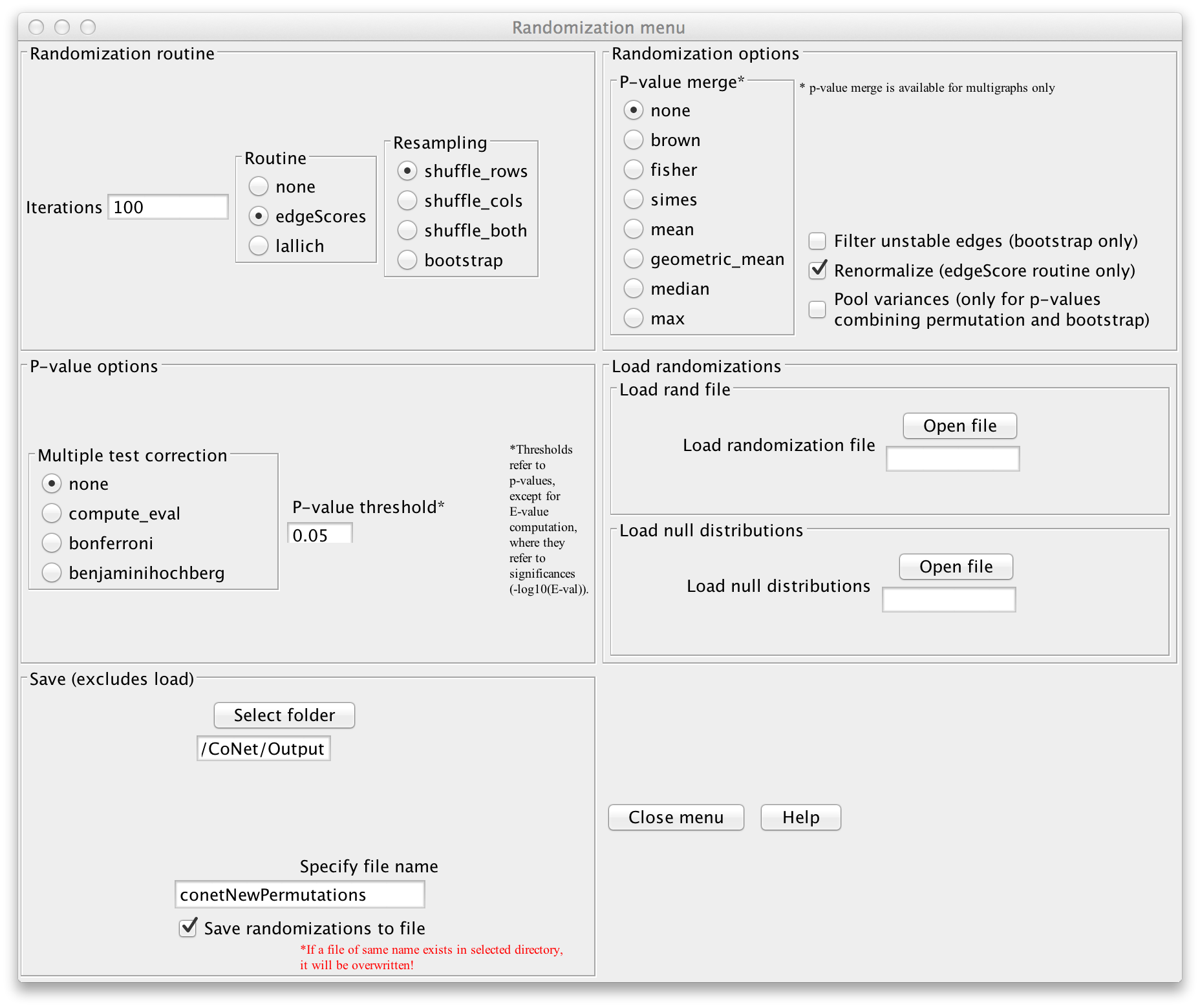
Else, open the "Randomization menu" and select "edgeScores" as routine and "shuffle_rows"
as resampling strategy. Enable "Renormalize" (this will shift the permutation
distribution such that compositionality biases are mitigated, as described in
PLoS Computational Biology 8 (7), e1002606. Select a folder in which the permutation file will be stored.
You can then enter a name for the permutation file (we will call it "conetNewPermutations.txt")
and enable "Save randomizations to file".
Click "GO" in the main menu to launch the computation. You can delete the intermediate network that appears
when computation is finished.
Step 4 - Bootstrapping
Final p-values are computed from method- and edge-specific permutation and
bootstrap score distributions. Thus, we will now compute the bootstrap distribution.
You can skip the bootstrap step (which takes 5 minutes to run) by downloading and unzipping the
conetNewBootstraps.txt.zip file. The next
step explains how to obtain networks from precomputed permutations and bootstraps.
If you want to use a configuration file for the bootstrap step, please download the
conet-boot-settings.txt file and load it
the same way as the permutation settings file. After adjustment of paths to input files and enabling
"Biom file in HDF5 format" in the Data menu, you also need to adjust the path to the permutation file
given in the randomization menu.
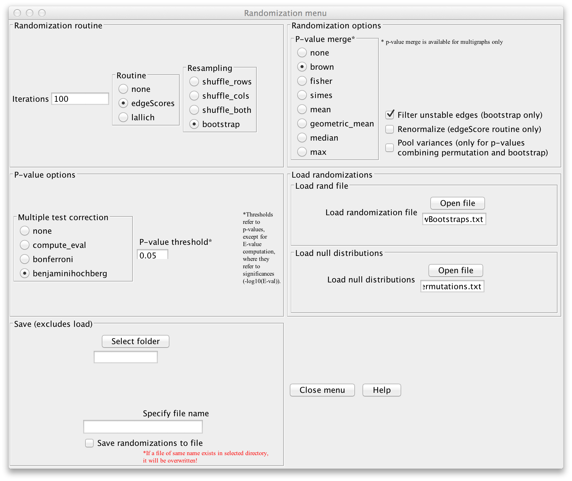
If you want to configure CoNet manually, open the randomization menu, select "bootstrap"
as resampling method and choose "brown" as p-value merge strategy. In the permutation step,
we computed method- and edge-specific p-values, but for the final network, we will merge
all method-specific p-values of an edge into one p-value using Brown's method
(Biometrics 31 (4) 987-992, 1975).
Disable "Renormalize" and enable "Filter unstable edges", which discards edges with original
scores outside the 0.95 range of their bootstrap distribution. You can then enable
the "benjaminihochberg" multiple testing correction. The permutation file can be loaded via
"Load null distributions". The bootstraps can be saved into a file by selecting a folder
in the "Save" section, then specifying a file name (we use "conetNewBootstraps.txt") and enabling
"Save randomizations to a file".

Click "GO" in the main menu to launch the computation. You have now computed the final network.
Optional Step 5 - Restore network from random files
Here we show how to restore a network from precomputed permutation and bootstrap files.
For this, either load the settings in the conet-restore-settings.txt
file as described previously (taking care to adjust the paths to all input and random files and to enable
"Biom file in HDF5 format" in the Data menu) or open the
Randomization menu, select "edgeScores" as routine, "bootstrap" as resampling strategy,
disable "Renormalize" and "Save randomizations", enable "Filter unstable edges" and empty the "Select folder"
and "file name" fields in the "Save" section.
You can then choose a p-value merge technique (we propose "brown") and a multiple-test correction
method (e.g. "bejaminihochberg").
We then load the previously computed permutations as null distribution and the bootstraps as
random distribution.
Click "GO" in the main menu to launch the computation. You have now (re-)computed the final network.
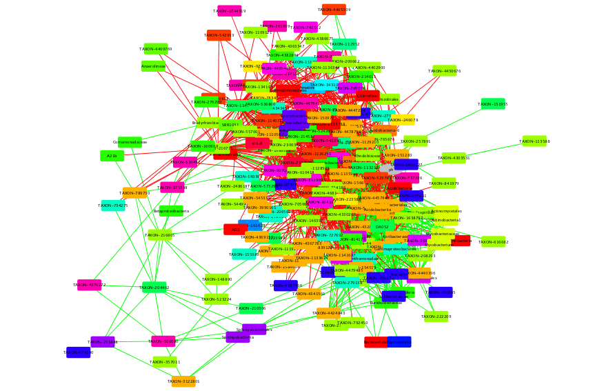
Step 6 - Visualization
First, you can select a network layout, e.g. Layout->yFiles Layouts->Organic.
CoNet returns a network with its own style, where positive and negative edges are colored
green and red, respectively. We can enhance the default style for instance by assigning
colors to different classes. For this, open the Style panel for Node, select
"Fill Color" with "class" as Column and choose "Discrete Mapping" as Mapping Type.
You can right-click on "Mapping Type", select "Mapping Value Generators", then "Rainbow"
to fill the different nodes with randomly selected class-specific colors.