LSA
LSA stands for local similarity analysis. Besides its original implementation in the
Sun lab, it has also been implemented in the
Hallam lab.
This tutorial will work with the second implementation, which is easier to install.
The core idea of the local similarity analysis is to carry out a local alignment on time series,
where correlations between OTUs may be shifted. Although our data set does not consist of
time series, we use LSA here for demonstration purposes. For more details on LSA, please
read the original publication in Bioinformatics 22(20),
2532-2538 2006, as well as the more recent publications in
Bioinformatics 29(2), 230-237 2012 (LSA)
and BMC Genomics 14(1) S3 2013 (fastLSA).
Step 1 - Run LSA
Please choose the input file "arctic_soils_filtered.txt".
fastLSA is a program that needs to be run on command line. You can launch it
with the following command:
./fastLSA -i arctic_soils_filtered.txt -o arctic_soils_lsa.txt -d 3 -a 0.01 > lsa.log
where -d is the maximum delay between time series (here chosen for demonstration) and alpha
the level of significance.
Step 2 - Visualize results
The output of fastLSA is a table with source and target nodes as well as additional node
attributes that can be loaded into Cytoscape using File->Import->Network->File.
Please select the first column as source node column and the second as target node column.
Column names can be changed by right-click. Make sure to select also the other columns
(including LSA values, lag, and p-values), which will be loaded as edge attributes.
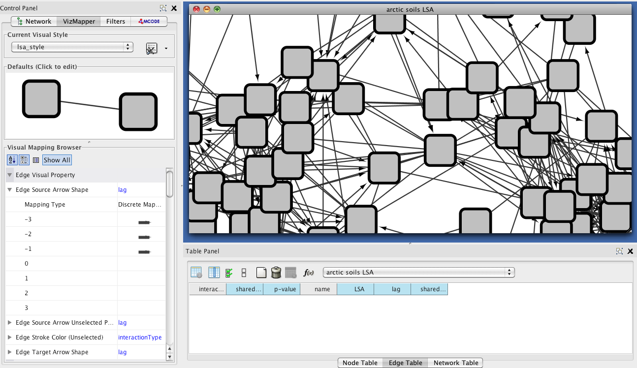
You can then layout the network using option Layout->yFiles Layouts->Organic and create
a LSA-specific style by copying the current visual style in the VizMapper.
For demonstration purposes, LSA was run with a delay of 3 (-d 3). Thus, we can assign directed
edges for lags unequal to zero using the Edge Source and Target Arrow shape visual properties
on the lag edge attribute (DiscreteMapping). We end up with a network that contains directed as well as undirected
edges.